Introduction

Don’t Decay the Learning Rate, Increase the Batch Size by Smith et al. offers a new technique for optimizing neural networks with stochastic gradient descent. It is common practice in machine learning to decrease the learning rate parameter in a neural network as epochs progress. Smith et al. show, through mathematical analysis, that the reason that this technique works is similar to the process of simulated annealing. Stochastic gradient descent produces “fluctuations” in the weights of the network, with higher learning rates leading to more severe fluctuations. Decreasing the learning rate over time decreases the size of the fluctuations as well. These fluctuations help the optimization process escape from local minima early in the training procedure, but the decreasing fluctuation size ensures that the network can settle into a minimum before the training ends, which is exactly how simulated annealing works.

Smith et al. suggest an alternative way of optimizing stochastic gradient descent based on this analysis. Since decreasing the learning rate works by decreasing the size of fluctuations, other methods of decreasing fluctuation size should also be effective. One way to decrease the size of fluctuations, they show, is to increase the size of batches over time. In fact, in most circumstances, a decrease in the learning rate by a certain factor is equivalent to multiplying the batch size by the same factor, in terms of the effect on fluctuation size. Therefore, a schedule designed for decaying learning rate can be easily transformed (by simply taking the inverse) to be directly usable as a schedule for increasing batch size, and the results should be the same.

This hypothesis is confirmed in the experiments in Smith et al.’s paper, at least for the architectures and datasets they used. They use large ResNet architectures with the CIFAR-10 and ImageNet databases, and find almost identical results when using a decreasing learning rate and increasing batch size.

Increasing the batch size is a preferable alternative to decreasing the learning rate because it leads to better performance. Increasing the batch size does not involve changing the parameters of the network, so using an increasing batch size instead of a decreasing learning rate involves significantly fewer parameter updates. Additionally, using larger batch sizes makes the training process more parallelizable.

The goal of this project is to confirm their results for simpler architectures and smaller datasets. In particular, I will make use of several different small architectures and the MNIST database of hand-written digits.

Methods

To replicate the results of this paper, I used the Keras API in TensorFlow with Python 3.

Smith et al. were using very large architectures like ResNet-50 and training on very complicated datasets like ImageNet, and thus used hundreds of training epochs. This project, however, is using smaller architectures and the MNIST database, which is much simpler. Therefore, I used only 12 epochs for training, because adding more epochs did not help performance at all due to the simplicity of the networks and the data.

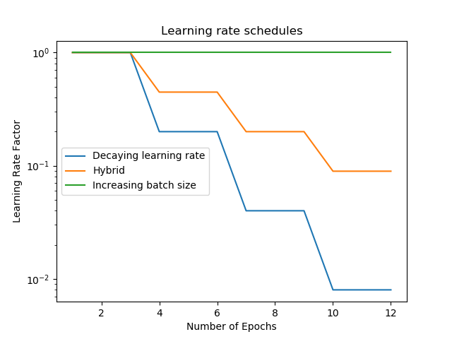
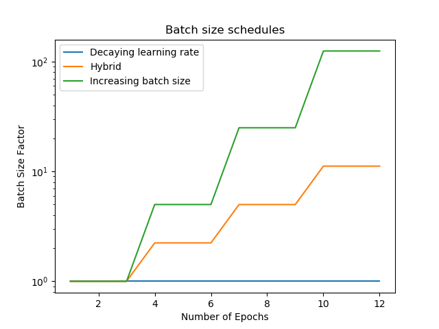
In their paper, Smith et al. use a learning rate decay schedule with 4 stages, such that the learning rate in each stage is smaller than the rate in the previous stage by a factor of 5. Inversely, in the schedule for increasing batch size, the batch size increases each stage by a factor of 5. I designed an analogous schedule for my experiments, with each stage containing 3 epochs.

In addition to training once by only decreasing the learning rate, and once by only increasing the batch size, Smith et al. include a hybrid approach where the learning rate and batch size change over time, by smaller amounts. I included a training approach like this as well. For this third hybrid approach, in each stage, the learning decreases by a factor of the square root of 5, and the batch size increases by a factor of the square root of five (batch size is rounded to the nearest whole number).



I tested these training schedules with three different network architectures. The first two are both simple neural networks consisting of normal dense matrix layers. The first has a single hidden layer with 300 units, while the second has two hidden layers with 500 units in the first and 150 in the second. These values were taken from this page which describes these architectures as being capable of achieving good results on the MNIST dataset. The final architecture is the LeNet-5 architecture, a convolutional neural network designed specifically for in recognizing hand-written digits by LeCun et al.

Each architecture was tested with all three training schedules (decreasing learning rate, increasing batch size, and hybrid). Additionally, following the paper by Smith et al., I tested each architecture with two different types of optimization. First, I used normal stochastic gradient descent with no momentum. Second, I used a more sophisticated optimization process called Adam developed by Kingman and Ba (2014).

Results

I tested three different architectures, and for each architecture I tested three different training procedures (decreasing learning rate, increasing batch size, and hybrid) and two different optimizers (normal stochastic gradient descent and Adam). The results of these tests are visible in the following images:







The results here are largely the same as those found in the Smith et al. paper: the learning curves from the decreasing learning rate procedure are identical to the curves from the increasing learning rate procedure (and the hybrid procedure). The lines for Architectures 1 and 2 are almost indistinguishable, however for Architecture 3 there is a small, but visible difference. This small difference may suggest that the result that Smith et al. found when training on the large ImageNet and CIFAR-10 datasets does not perfectly translate to this context. This small difference was persistent over several trials with varying initial weights.

Interestingly, these results are somewhat mixed in that when using SGD optimization on Architecture 3, increasing batch size produced better a accuracy than decreasing learning rate, but when instead using Adam optimization on the same architecture, the opposite occurred. This suggests that the difference in the optimization procedure may be more important than the difference between increasing batch size and decreasing learning rate, in the context of this project.

References

Don’t Decay the Learning Rate, Increase the Batch Size by Smith et al. (2018). This is the main paper I was aiming to replicate.

This page describes the performance of many different architectures on the MNIST database, and is where I drew the shapes for the first two architectures I used.

Gradient-Based Learning Applied to Document Recognition by LeCun et al. (1998). This paper describes LeNet-5, which is the third architecture I tested in this project.

Adam: A Method for Stochastic Optimization by Kingman and Ba (2014). This paper describes the Adam optimization procedure used in half of the tests in this project.

Coupling Adaptive Batch Sizes with Learning Rates by Balles et al (2016). This paper investigates the relationship between learning rate and batch size for optimization by stochastic gradient descent. This paper provides background for the theoretical work done in Don’t Decay the Learning Rate, Increase the Batch Size, the main paper for this project.

Code

The code I wrote for this project is contained in two scripts: main.py, which does most of the work involved with the project including defining the architectures and running all the training procedures while measuring accuracy, and plots.py which uses the data computed by main.py to produce the graphs that appear in this paper. main.py computes the accuracies and then pickles the dictionary that contains them, and the pickled file is then read by plots.py, so to reproduce my results, you should place main.py and plots.py in the same directory, then run main.py, and finally run plot.py.